![Validation and Optimization: tuning parameters for the implicit H-bond interaction method using datasets [GSoC 2025 - Week 10]](/images/blog_pics/gsoc-wk-10.png)
Hello, welcome to blog post on the week 10 of my GSoC journey! From the last blog post, we completed the development of the implicit H-bond interaction class. However, it is not perfect. Before getting this method merged into the main ProLIF, we have to validate our method using the explicit H-bond method. Thus we used a dataset, PLINDER, to achieve this.
In this blog post, you will learn how we validated our implicit H-bond method and understand what parameters were tuned.
How to validate our method?
We used explicit H-bond interaction method as ground truth to validate our method using a protein-ligand complex. Here are the steps:
- Protonate the protein and add hydrogens for the ligand.
- Calculate explicit H-bond interactions.
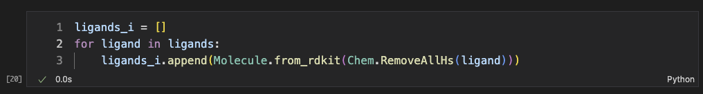
- Remove the hydrogens in the ligand and protein, and then calculate implicit H-bond interactions (our method).
- Compare donor-acceptor pairs from explicit and implicit H-bond methods.
An example
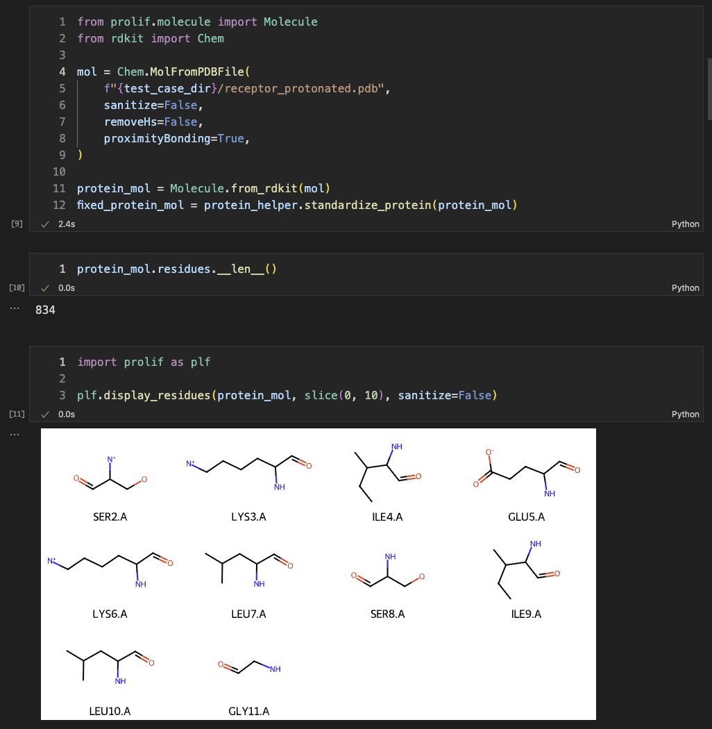
First, for protein protonation, we used PDB2PQR (PROPKA3) and reduce (if PDB2PQR is not working for the system). For adding hydrogens for ligands, I used openbabel. See how we dealt with a lot of data: click here.
Then, we read the protein with RDKit, converted it into prolif.Molecule, and fixed bond orders with our ProteinHelper. The ligand was also read as a prolif.Molecule.
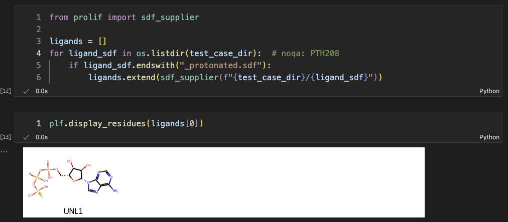 It is noted that multiple ligands can interat with a single protein. We used a list to save all possible ligands for that protein receptor.
Next, we calculated the explicit H-bond interations with default parameters (distance = 3.5 Å, D-H-A angle is between 130° and 180°). They were considered as ground-truth H-bond interactions for this protein-ligand system.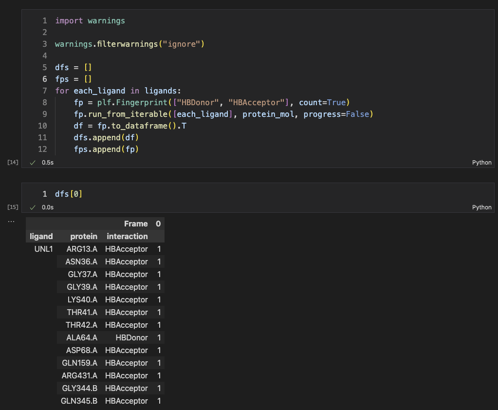
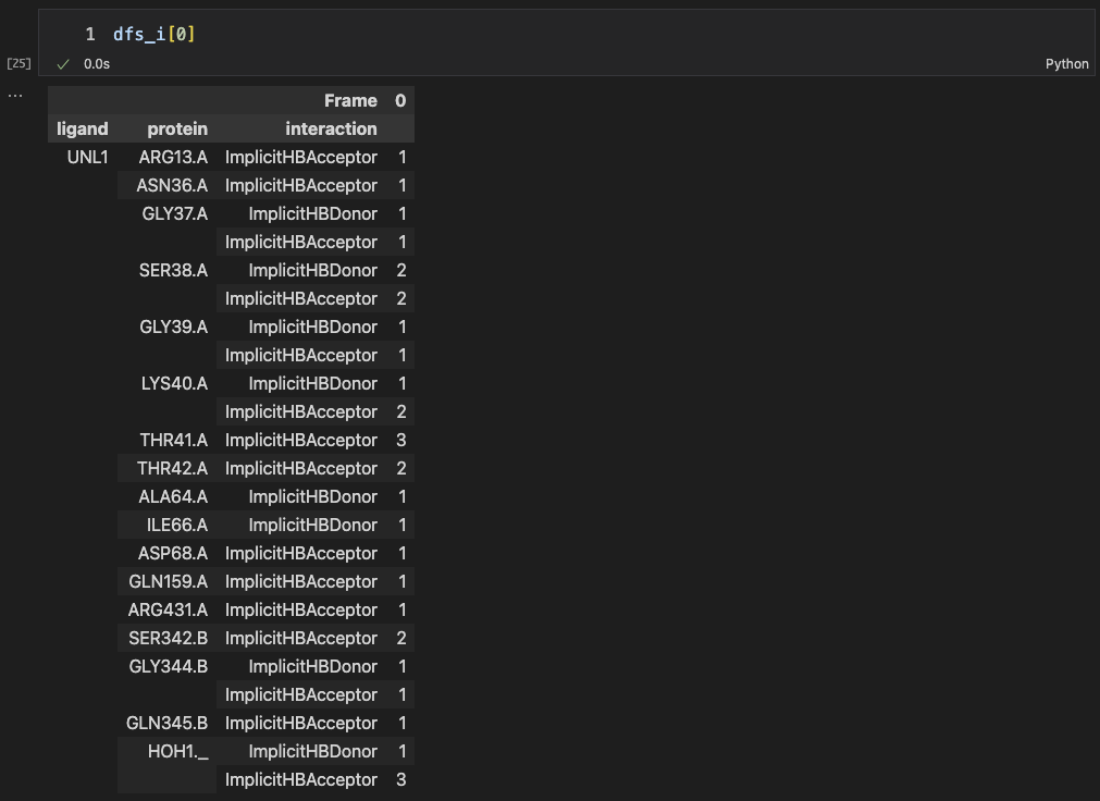
The above results show the interaction pairs between the ligand and residues.
Then, we can also do the same thing for implicit H-bond method. We used RDKit to remove the explicit hydrogens before ProteinHelper.
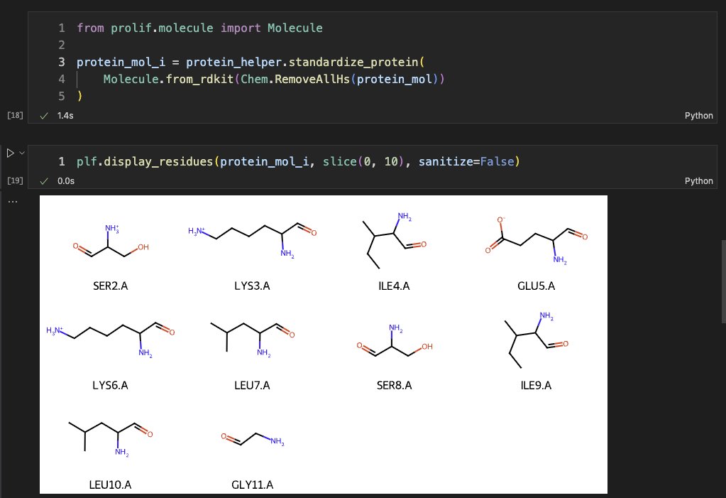
Same for the ligand, we removed the explicit hydrogens.
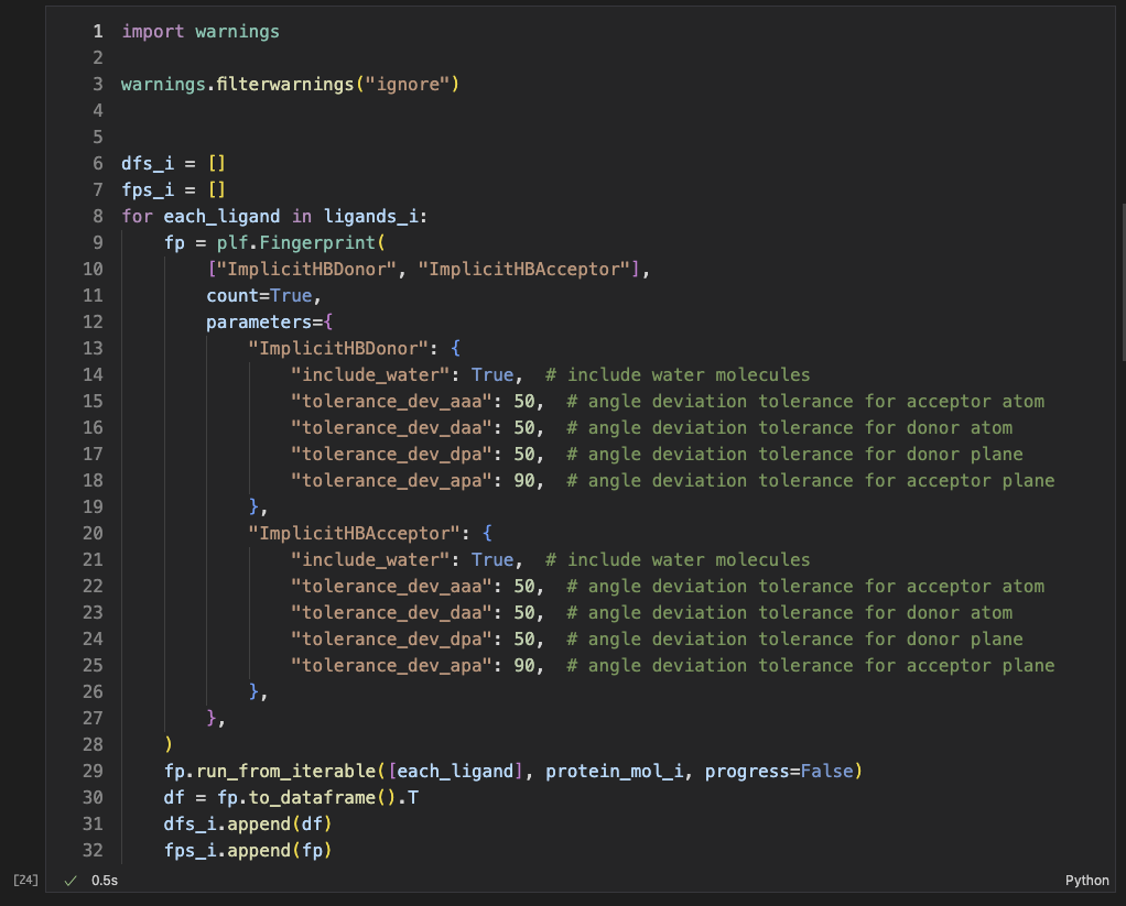
For the calculation of the implicit H-bond interations, we included water molecules. Also, we set a relatively large tolerance for each deviation of atom/plane angles so that we wouldn’t miss any possible pairs from the explicit methods (yes, we intentionally minimized false negatives but it might generate lots of false positives).
Here is the list of interaction pairs from implicit H-bond method.
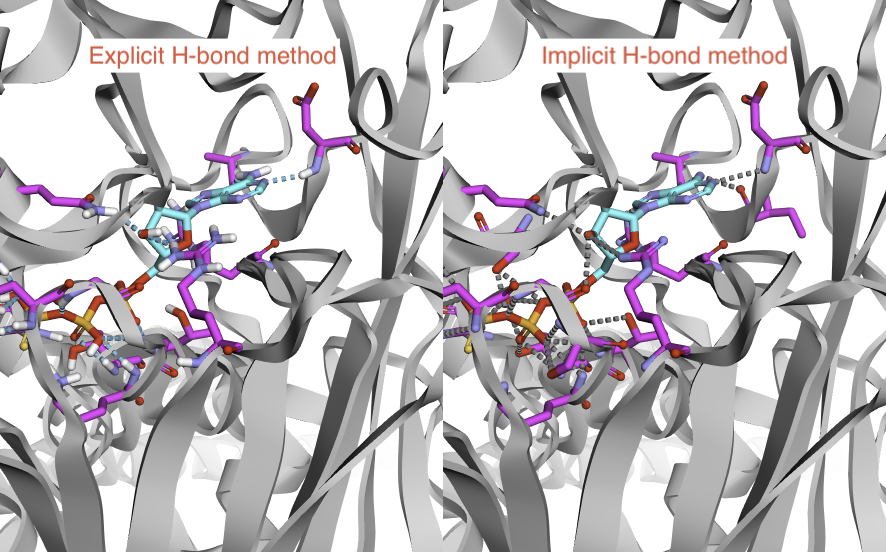
Finally, we compared the different sets of interaction pairs from implicit and explicit methods. In implicit H-bond method, 23 interactions are detected. However, only 13 interactions are actually detected by the explicit H-bond method.

We also calculated “Tanimoto coefficient” (or said Jaccard index, or simply Intersection over Union (IoU)) between two methods.
Tanimoto = 13 / (13 + 10 + 0) ~= 0.565
Now, we had a quatitative method to compare interaction pairs from two differnt methods (not only maunally visulization like the below picture).
Tuning the implicit H-bond parameters
The next thing to think about is:
How do we improve the accuracy of our method?
In the implicit H-bond methods, we have several parameters, including acceptor atom angle deviation, donor atom angle deviation, acceptor plane angle, donor plane angle. If we know how to set a good threshold for each parameter, we can have more accurate results. To achieve this, we would like use the power of datasets.
Our goal is to analyze all hydrogen bond interaction pairs identified using the explicit hydrogen bond method in the dataset (we used PLINDER dataset). Specifically, we examined the distribution of geometric parameters (acceptor atom angle deviation, donor atom angle deviation, acceptor plane angle, donor plane angle). Additionally, we compared these “ground-truth” H-bond pairs with false positives generated by the implicit H-bond method to determine whether their distribution profiles differ significantly. In the end, we can decide cutoff values for each geometric parameters (that is why we called parameter tuning).
PLINDER dataset
PLINDER is a protein-ligand dataset with mutliple annotations. The dataset was splitted into training (n~=420K), validation (n=1157) and testing (n=1436) sets to minimize leakage and maximize the quality of test.
For our parameter tuning, we used PLINDER’s validation set as our first dataset to investigate the parameters’ distribution, and PLINDER’s testing set for testing the selection of the parameters.
Donor and acceptor atom angle deviation’s distribution
The points represent each interaction pair’s acceptor atom angle deviation and donor atom angle deviation in the PLINDER’s validation set (overall averaged Tanimoto coefficient: 0.565). The blue one is detected by both implicit and explicit H-bond methods while the red one is detected by the implicit H-bond method only. From the distribution of the acceptor atom angle deviation, two sets are identical. This suggests that we cannot select a cutoff of this parameter to reduce the false positives. However, we can select a cutoff value of 25° for the donor atom angle deviation. Because lots of false positives have a greater donor atom angle deviation compared to the ground truth.
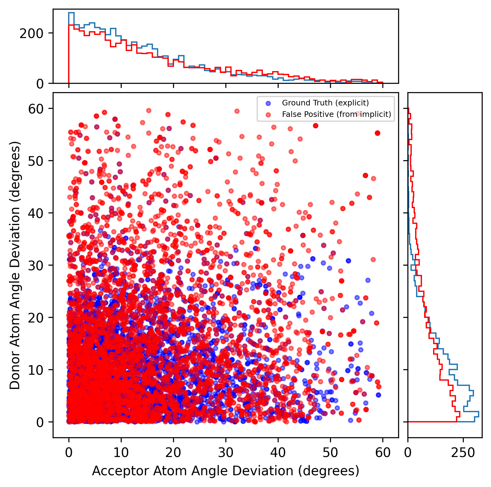 It is noted that the tolerance of atom angle deviation was originally set in 60°. There are 14 (~1%) protein-ligand system fails to detect H-bond interactions wither from the explicit or implicit methods due to computing errors (under investigation).
Donor and acceptor plane angles’ distribution
We did a similar analyses for plane angles. Interesting, the acceptor plane angles again show no difference between the ground truths and the false positives. But, we can set a donor plane angle of 30° to reduce false positives.
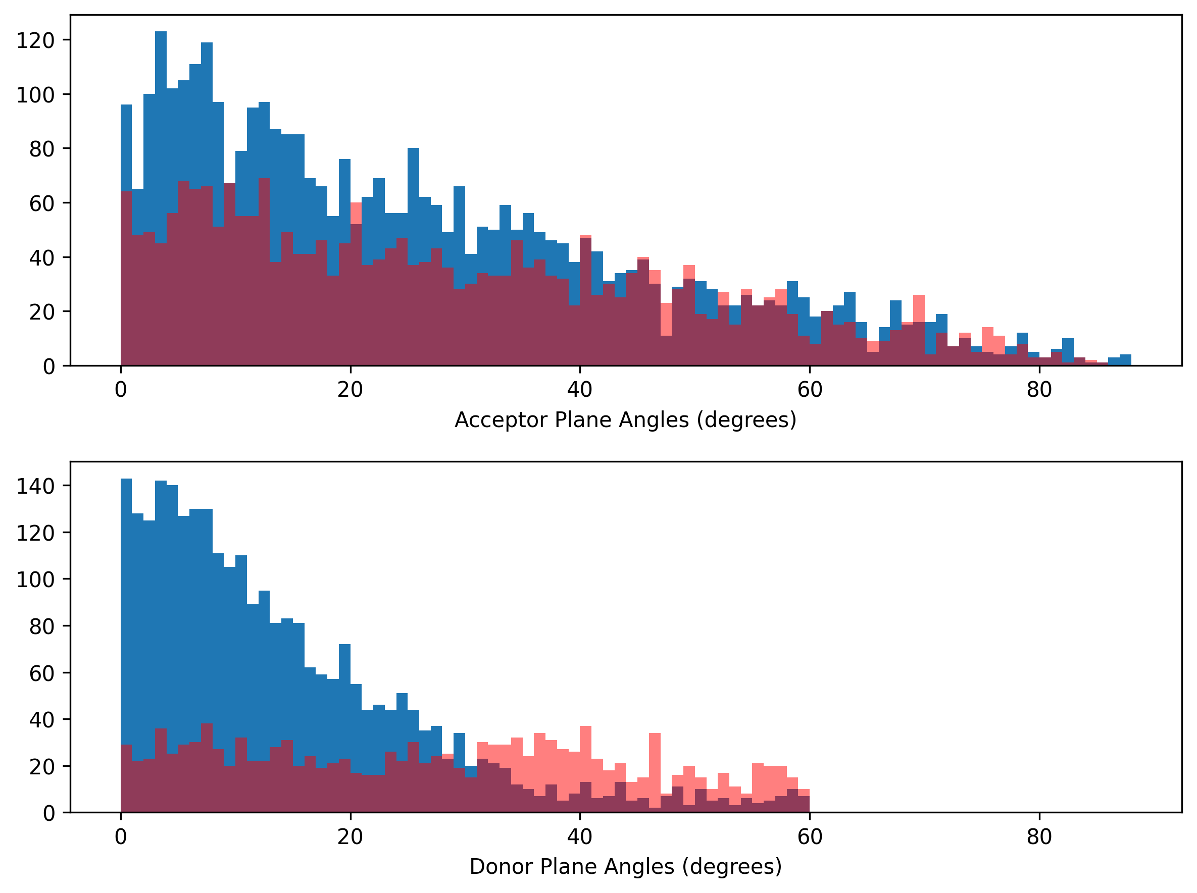 It is noted that the tolerance of acceptor and donor plane angles was originally set in 90° and 60°, respectively. There are 14 (~1%) protein-ligand system fails to detect H-bond interactions wither from the explicit or implicit methods due to computing errors (under investigation).
Summary
Now, we have found the cutoff values for some parameters in the implicit H-bond interaction method.
- Tolerance of acceptor atom angle deviation: it doesn’t matter.
- Tolerance of donor atom angle deviation: 25°.
- Tolerance of acceptor plane angle: it doesn’t matter.
- Tolerance of donor plane angle: 30°.
We will next finalize our functions and it will then be ready to go.
See you in the next blog post.
More about GSoC 2025: MDAnalysis x ProLIF project 5
See how we manage this project: click on this [link]. The code for the validation shown in the blog post is also in the same repo. If you want to know more about the project’s details, you can find it via GSoC Project Page or ProLIF Github.
Note: The top picture was generated by Flux Pro 1.1 Ultra with Oil Painting style, aspect ratio: 16:9, generation count 4 (I picked one picutre out of four.), and prompts: “I would like a drawing with the idea of the below keywords but no texts: implicit hydrogen versus explicit hydrogen, geometrical constraints, coding for cheminformatics, molecule, parameters tuning, using datasets, Protein-Ligand interaction, Protonation tools.”.